Pareto distribution
Probability density function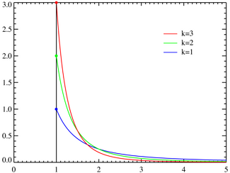 Pareto probability density functions for various α with xm = 1. The horizontal axis is the x parameter. As α → ∞ the distribution approaches δ(x − xm) where δ is the Dirac delta function. |
|
Cumulative distribution function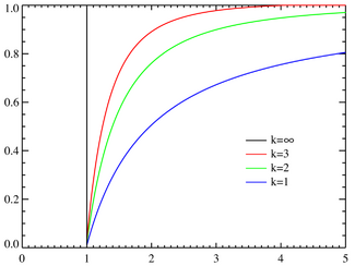 Pareto cumulative distribution functions for various α with xm = 1. The horizontal axis is the x parameter. |
|
| parameters: |  scale (real) scale (real) shape (real) shape (real) |
|---|---|
| support: |  |
| pdf: | 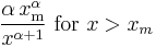 |
| cdf: |  |
| mean: |  |
| median: | ![x_\mathrm{m} \sqrt[\alpha]{2}](/I/3c52a1728ced91e276d35d6e39be8ac3.png) |
| mode: |  |
| variance: |  |
| skewness: |  |
| ex.kurtosis: |  |
| entropy: |  |
| mgf: |  |
| cf: |  |
| Fisher information: |  |
The Pareto distribution, named after the Italian economist Vilfredo Pareto, is a power law probability distribution that coincides with social, scientific, geophysical, actuarial, and many other types of observable phenomena. Outside the field of economics it is at times referred to as the Bradford distribution.
Pareto originally used this distribution to describe the allocation of wealth among individuals since it seemed to show rather well the way that a larger portion of the wealth of any society is owned by a smaller percentage of the people in that society. This idea is sometimes expressed more simply as the Pareto principle or the "80-20 rule" which says that 20% of the population controls 80% of the wealth[1]. The probability density function (PDF) graph on the right shows that the "probability" or fraction of the population that owns a small amount of wealth per person is rather high, and then decreases steadily as wealth increases. This distribution is not limited to describing wealth or income, but to many situations in which an equilibrium is found in the distribution of the "small" to the "large". The following examples are sometimes seen as approximately Pareto-distributed:
- The sizes of human settlements (few cities, many hamlets/villages)
- File size distribution of Internet traffic which uses the TCP protocol (many smaller files, few larger ones)
- Clusters of Bose–Einstein condensate near absolute zero
- The values of oil reserves in oil fields (a few large fields, many small fields)
- The length distribution in jobs assigned supercomputers (a few large ones, many small ones)
- The standardized price returns on individual stocks
- Sizes of sand particles
- Sizes of meteorites
- Numbers of species per genus (There is subjectivity involved: The tendency to divide a genus into two or more increases with the number of species in it)
- Areas burnt in forest fires
- Severity of large casualty losses for certain lines of business such as general liability, commercial auto, and workers compensation.
Properties
Definition
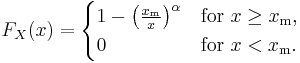
If X is a random variable with a Pareto distribution, then the probability that X is greater than some number x is given by
where xm is the (necessarily positive) minimum possible value of X, and α is a positive parameter. The family of Pareto distributions is parameterized by two quantities, xm and α. When this distribution is used to model the distribution of wealth, then the parameter α is called the Pareto index.
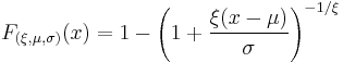
It follows from the above that therefore the cumulative distribution function of a Pareto random variable with parameters α and xm is
Density function
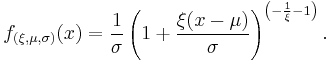
It follows (by differentiation) that the probability density function is
![f_X(x)= \begin{cases} \alpha\,\dfrac{x_\mathrm{m}^\alpha}{x^{\alpha+1}} & \text{for }x > x_\mathrm{m}, \\[12pt] 0 & \text{for } x < x_\mathrm{m}. \end{cases}](/I/b61e8288e0eae52f572a05d5117795df.png)
Moments and characteristic function
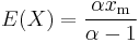
- The expected value of a random variable following a Pareto distribution with α > 1 is
-
- (if α ≤ 1, the expected value does not exist).
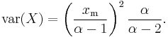
- The variance is
-
- (If α ≤ 2, the variance does not exist).
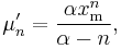
- The raw moments are
-
- but the nth moment exists only for n < α.
- The moment generating function is only defined for non-positive values t ≤ 0 as

- The characteristic function is given by
-
- where Γ(a, x) is the incomplete gamma function.

Degenerate case
The Dirac delta function is a limiting case of the Pareto density:
Conditional distributions
The conditional probability distribution of a Pareto-distributed random variable, given the event that it is greater than or equal to a particular number x1 exceeding xm, is a Pareto distribution with the same Pareto index α but with minimum x1 instead of xm.
Relation to the exponential distribution
The Pareto distribution is related to the exponential distribution as follows. If X is Pareto-distributed with minimum xm and index α, then
is exponentially distributed with intensity α. Equivalently, if Y is exponentially distributed with intensity α, then

is Pareto-distributed with minimum xm and index α.
A characterization theorem
Suppose Xi, i = 1, 2, 3, ... are independent identically distributed random variables whose probability distribution is supported on the interval [xm, ∞) for some xm > 0. Suppose that for all n, the two random variables min{ X1, ..., Xn } and (X1 + ... + Xn)/min{ X1, ..., Xn } are independent. Then the common distribution is a Pareto distribution.
Relation to Zipf's law
Pareto distributions are continuous probability distributions. Zipf's law, also sometimes called the zeta distribution, may be thought of as a discrete counterpart of the Pareto distribution.
Pareto, Lorenz, and Gini
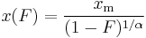
The Lorenz curve is often used to characterize income and wealth distributions. For any distribution, the Lorenz curve L(F) is written in terms of the PDF ƒ or the CDF F as
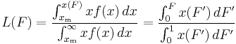
where x(F) is the inverse of the CDF. For the Pareto distribution,
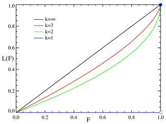
and the Lorenz curve is calculated to be
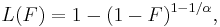
where α must be greater than or equal to unity, since the denominator in the expression for L(F) is just the mean value of x. Examples of the Lorenz curve for a number of Pareto distributions are shown in the graph on the right.
The Gini coefficient is a measure of the deviation of the Lorenz curve from the equidistribution line which is a line connecting [0, 0] and [1, 1], which is shown in black (α = ∞) in the Lorenz plot on the right. Specifically, the Gini coefficient is twice the area between the Lorenz curve and the equidistribution line. The Gini coefficient for the Pareto distribution is then calculated to be
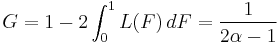
(see Aaberge 2005).
Parameter estimation
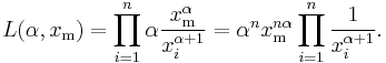
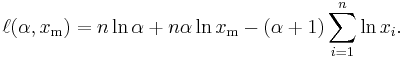
The likelihood function for the Pareto distribution parameters α and xm, given a sample x = (x1, x2, ..., xn), is
Therefore, the logarithmic likelihood function is
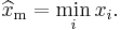
It can be seen that  is monotonically increasing with
  , that is, the greater the value of , the greater the value of the likelihood function. Hence, since
  , we conclude that
To find the estimator for α, we compute the corresponding partial derivative and determine where it is zero:
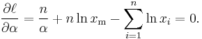
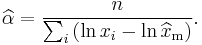
Thus the maximum likelihood estimator for α is:
The expected statistical error is:

Graphical representation
The characteristic curved 'long tail' distribution when plotted on a linear scale, masks the underlying simplicity of the function when plotted on a log-log graph, which then takes the form of a straight line with negative gradient.
Generating a random sample from Pareto distribution
Random samples can be generated using inverse transform sampling. Given a random variate U drawn from the uniform distribution on the unit interval (0, 1), the variate

is Pareto-distributed.
Bounded Pareto distribution
The bounded Pareto distribution has three parameters α, L and H. As in the standard Pareto distribution α determines the shape. L denotes the minimal value, and H denotes the maximal value. (The Variance in the table on the right should be interpreted as 2nd Moment).
| parameters: |  location (real) location (real)
|
|---|---|
| support: |  |
| pdf: |  |
| cdf: |  |
| mean: |  |
| median: |  |
| mode: | |
| variance: |  |
| skewness: | |
| ex.kurtosis: | |
| entropy: | |
| mgf: | |
| cf: |
 location (
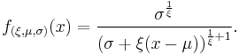
The probability density function is
where  , and α > 0.
Generating bounded Pareto random variables
If U is uniformly distributed on (0, 1), then
is bounded Pareto-distributed[3]
Generalized Pareto distribution
The family of generalized Pareto distributions (GPD) has three parameters  and
and  .
.
| parameters: |  location (real) location (real)
|
|---|---|
| support: | 
|
| pdf: |  where |
| cdf: |  |
| mean: |  |
| median: |  |
| mode: | |
| variance: |  |
| skewness: | |
| ex.kurtosis: | |
| entropy: | |
| mgf: | |
| cf: |
 scale (real)
 shape (real)

The cumulative distribution function is
for  , and
, and  when
when  , where
  is the location parameter,
  the scale parameter and
  the shape parameter. Note that some references give the "shape parameter" as
  .
.
The probability density function is:
or
again, for , and when .
Generating generalized Pareto random variables
If U is uniformly distributed on (0, 1], then
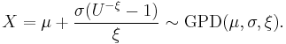
In Matlab Statistics Toolbox, you can easily use "gprnd" command to generate generalized Pareto random numbers.
See also
- Pareto analysis
- Pareto efficiency
- Pareto interpolation
- Pareto principle
- The Long Tail
- Traffic generation model
Notes
References
- Lorenz, M. O. (1905). Methods of measuring the concentration of wealth. Publications of the American Statistical Association. 9: 209–219.
External links
- The Pareto, Zipf and other power laws / William J. Reed -- PDF
- Gini's Nuclear Family / Rolf Aabergé. -- In: International Conference to Honor Two Eminent Social Scientists, May, 2005 -- PDF
|
||||||||||||||||||||||||||||||||||||||||||||||||||||||||||||||||||
|
|||||||||||